RESEARCH
September 2020
Kay Robbins1 Senior Member, IEEE and Tim Mullen2, Member IEEE
1University of Texas at San Antonio, 78249, USA (kay.robbins@utsa.edu).
2Intheon, San Diego, CA 92121
Although electroencephalography (EEG) is an important high time-resolution brain imaging technology used in laboratory, clinical, and even consumer applications, consistent handling of signal artifacts continues to be an important challenge. In a recent series of papers [1] [2] [3], we and collaborators compared EEG analysis results across multiple studies, EEG headset types, and preprocessing methods. We considered channel and source signal characteristics and explored time-locked event analysis. The work produced several insights of general interest to EEG researchers, as outlined below.
EEG preprocessing usually has several distinct phases including removal of line noise, referencing the signal, identification and removal or interpolation of bad channels, and identification and removal of ocular and other artifacts. Each of these stages influences signal statistics, but the methods used vary widely across studies. The big questions are how much of a difference do these choices make in the end results and what is the “best” preprocessing approach?
Our recent work reported in Robbins et al. [1] addresses these issues by comparing several approaches in a large-scale study. We looked at 18 studies in two general categories with many variations: target detection and driving with lane-keeping [2], analyzing over 1000 EEG recordings from five laboratory-grade EEG recording systems made by Biosemi (3 headset types) and Neuroscan (2 headset types). We compared results from two pairs of preprocessing strategies. One pair of methods was based on independent component analysis (ICA) artifact removal, the other pair was based on artifact subspace reconstruction (ASR). (The details can be found in [1] and two related papers [2][3] and are not reported here.)
Our bottom line answer to the first question is that the early stage preprocessing choices influence end results at all levels, sometimes in significant ways. Our answer to the second question is that there is likely no single “best” approach, but rather a portfolio of good choices. Rather than pick one approach, research studies should characterize the variability introduced by different choices as part of the reporting process. These studies also have several other take-away points that we briefly summarize here.
Scaling by a recording-specific constant reduces inter-subject variability
Our work has demonstrated that regardless of the headset or the preprocessing method, scaling each recording by a recording-specific constant reduces variability of results across recordings by roughly 40%. Scaling is particularly important when combining datasets for joint analyses and improves comparability when presenting results from multiple datasets [1]. Statistically, we found that scaling using the Huber mean[1] produced the greatest reduction in variability. We note that scaling should be performed after artifact removal. We hypothesize that this improvement is due to the indirect relationship between EEG signal amplitude in the brain and the measurement scale used in each EEG recording. The measurement scale depends on the equipment amplifiers and the voltage gain settings as well as the loss factor introduced by transmission through an individual subject’s skull, scalp and hair.
It’s in the eyes…
Unsurprisingly, raw EEG (or mildly preprocessed EEG with only filtering and bad channel identification and interpolation) has much higher amplitude in the frontal and occipital channels than more centrally located channels, mostly attributable to eye artifacts [1]. Eye artifact removal equalizes channel amplitudes across the scalp for all of the preprocessing methods we studied. However, our analysis shows that even after aggressive artifact removal, significant residual blink artifacts can remain that may not be visible through cursory data inspection.
To quantify blink residual, we define the blink amplitude ratio as the mean absolute value of the signal within [−0.5, 0.5] seconds around the blink maximum divided by the mean absolute value of the signal within [−1.5, −1] seconds and [1, 1.5] seconds from the blink maximum. If an artifact removal method has entirely removed a blink the resulting ratio should be near 1.0. The blink amplitude ratio can be computed either for epochs time-locked to the maxima of individual blinks or for blink ERPs (event-related potentials) computed by averaging these epochs. Note: ERPs can be computed either by averaging the time-locked blink epochs of a recording or by using linear regression (temporal overlap regression).
The gray boxplots in Fig. 1 show the distribution of blink amplitude ratios for individual epochs time-locked to the blink maxima of non-overlapping blinks. The blue boxplots show the amplitude ratios of the corresponding averaged blink ERPs. The two ICA-based methods are called LARG and MARA in the figure. The two ASR-based methods are called ASR_10* and ASR_5*. (See [1] for details.) MARA and the ASR-based methods have median ERP blink ratios much greater than 1, indicating a systematic bias. Artifact removal appears to take out too much signal around the blink max and not enough in the blink wings. On the other hand, LARG regresses out blinks in the intervals [−1, 1] around blink maxima. This aggressive removal appears to take out too much signal. Note: we also verified that pseudo ERPs calculated by averaging randomly selected intervals had blink amplitude ratios clustered tightly around 1.
Researchers should assume residual blink signals are present in their data after preprocessing and take active measures to address this when interpreting their results. Since neural activity has also been observed time-locked to spontaneous blinks, we recommend examining multiple factors, including the spatial and spectral distribution of residual activity locked to blinks, when characterizing the origin of this activity. Use of temporal overlap regression may also be preferable to event-related averaging by allowing researchers to regress out common patterns of activity unique to blink events and to compare results with and without blink events included in the design matrix. We additionally recommend that researchers use and carefully document their methods of outlier removal.
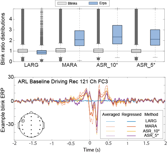
Fig. 1. Top: distribution of blink amplitude ratios for individual blinks (gray) and blink ERPs (blue) for non-overlapping blink epochs for different preprocessing methods LARG and MARA are ICA based, while ASR_10* and ASR_5* are ASR based methods. Dark gray crosses represent outliers. Bottom: example of an individual residual blink ERP, computed both by averaging and by temporal overlap regression, following artifact removal using various methods. The inset shows the electrode positions of the 26 common channels used for the top graph. FC3 is the circled electrode.
It pays to automate and to federate
Another point established in our work is that even relatively minor differences in EEG preprocessing can result in significant differences in derived measures [3]. To quantify these differences in the frequency domain we computed, for each pair of pre-processing methods, the pairwise correlation in spectral band power for 100 four-second samples taken at random from each channel and recording. Fig. 2 shows the distribution of correlations.

Fig. 2. Spectral sample vector correlations between pairs of preprocessing methods for different frequency bands.
The dark gray ‘bars’ in Fig. 2 are comprised of individual markers, each representing an outlier channel for a recording. Even in closely related methods such as ASR_5* and ASR_10* (which differ solely in the value of the burst cutoff parameter controlling aggressiveness of high-variance artifact removal), many individual recordings processed using different methods have low correlation.
Discussion
Identifying groups of preprocessing methods or parameters that consistently produce similar results across diverse and heterogeneous data can help in generalizing performance and establishing functional equivalency between methods. For methods that produce different results, the question stands: “which method is better?” Our experience has led us to conclude that attempting to produce a single “gold standard” for pre-processing may be infeasible or ill-advised. Instead, a diversity approach may lead to more reproducible and meaningful results. If a federation of automated processing pipelines with well-documented and standardized parameter choices were available, researchers could run their data through several of them and compare the results as part of reporting their research. Large differences in analysis output would be analyzed as part of the research reporting, leading to a better understanding both of the methods and the underlying neural phenomena.
References
[1] K. A. Robbins, J. Touryan, T. Mullen, C. Kothe, and N. Bigdely-Shamlo, “How sensitive are EEG results to preprocessing methods: A benchmarking study,” IEEE Trans Neural Syst Rehabil Eng, vol. 28, no. 5, pp. 1081–1090, May 2020, doi: 10.1109/TNSRE.2020.2980223. [2] N. Bigdely-Shamlo, J. Touryan, A. Ojeda, C. Kothe, T. Mullen, and K. Robbins, “Automated EEG mega-analysis I: Spectral and amplitude characteristics across studies,” NeuroImage, p. 116361, Nov. 2019, doi: 10.1016/j.neuroimage.2019.116361. [3] N. Bigdely-Shamlo, J. Touryan, A. Ojeda, C. Kothe, T. Mullen, and K. Robbins, “Automated EEG mega-analysis II: Cognitive aspects of event related features,” NeuroImage, p. 116054, Sep. 2019, doi: 10.1016/j.neuroimage.2019.116054.
[1] See https://github.com/VisLab/EEG-Pipelines for an implementation of the Huber mean function.
Author Biographies:

Tim Mullen holds M.S. and Ph.D degrees in cognitive sciences from UC San Diego, and B.A.s in computer science and cognitive neuroscience (highest honors) from UC Berkeley. He is a recipient of the UCSD ChancellorÕs Dissertation Medal, IEEE best paper awards, and various fellowships. His scientific research centers on computational neuroscience and applications of machine learning and signal processing to electrophysiological and other data to understand neural dynamics and brain network function and to decode mental states. Over the last decade, he has contributed extensively to open source software and standards initiatives for neuroscience data analysis and sharing, including the EEGLAB ecosystem. He is founding CEO and Research Director at Intheon, which is pioneering a software platform for neural/bioÊdata analytics and brain-computer interfacing.
 Kay Robbins (M’89–SM’04) holds B.S. and Ph.D. degrees in mathematics from the Massachusetts Institute of Technology, Boston, MA, USA. She is currently a Professor Emeritus in the Department of Computer Science at the University of Texas at San Antonio, San Antonio, TX, USA, where she continues work on large-scale analysis and visualization of scientific data, with particular interests in neuroscience. Her lab has developed many open-source tools for EEG analysis. She is also working closely with a community of researchers to develop and standardize methods and vocabulary for annotating experimental data suitable to large-scale analysis.